Next: Meteorological tide comparison. Up: Application over the Río Previous: Description.

Astronomic tide simulation.

The amplitude of the main semi-diurnal tidal component (M₂) inside the Río de la Plata oscillates among 0.30 m to 0.10 m approximately, being larger over the Argentinean coast. That is why it is classified as a micro-tidal regime. The tide surge takes about 12 hours to reach the interior limit. This makes that, at every moment, there exists a complete cycle of semi-diurnal component inside the Río de la Plata (Balay, 1961).

**Figure 8.1:** Velocity field corresponding to high-tide in Montevideo,
low-tide in Colonia.
Semi diurnal Astronomic component (M₂).
$\begin{figure} \par\begin{center} \par\mbox{\epsfig{file=subemont, width=0.95\textwidth} } % \par\end{center}\par\end{figure}$

**Figure 8.2:** Velocity field corresponding to low-tide in Montevideo,
high-tide in Colonia.
Semidiurnal Astronomic component (M₂).
$\begin{figure} \begin{center} \mbox{\epsfig{file=bajamont, width=0.95\textwidth} } % \par\end{center}\par\end{figure}$

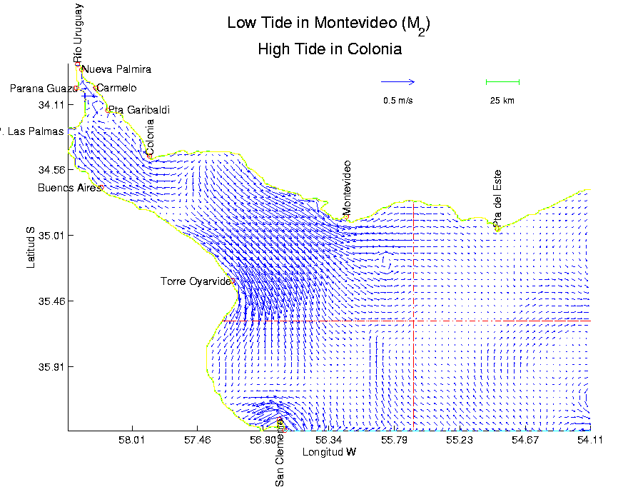Figures 8.1 and 8.2 show the velocity field in the Río de la Plata at two different instants, 6 hours (half wave period) apart in time from each other. Figure 8.1 represents the situation when the high-tide reaches Montevideo; figure 8.2 shows the velocity field when the low-tide arrives at Montevideo.

**Figure 8.3:** Level comparison.
Río de la Plata astronomic tide simulation, M₂ component.
$\begin{figure} \begin{center} \par\mbox{\epsfig{file=astrom2, width=0.95\textwidth} } % \par\end{center} \end{figure}$

**Figure 8.4:** Level comparison.
Río de la Plata astronomic tide simulation, 4 components.
$\begin{figure} \begin{center} \par\mbox{\epsfig{file=astro, width=0.95\textwidth} } % \par\end{center}\par\end{figure}$

**Figure 8.5:** Velocity field corresponding to high-tide in the upper Río de la Plata. Semi diurnal Astronomic component (M₂).
$\begin{figure} \begin{center} \mbox{\epsfig{file=subecolo, width=0.95\textwidth} } % \par\end{center}\par\end{figure}$

Figure 8.3 presents the calculated levels, considering only the main semi-diurnal component (M₂) of the astronomic surge, compared to real data, meteorological tide effects were neglected.

Figure 8.4 shows the water level of the 4 main components of the astronomic tide (M₂, N₂, K₁ and O₁, see table 8.1) compared to real wave data (obtained from Table des marées des grands ports du Monde (1983) and Almanaque 1987 (1986)).

As is shown in those figures there is a good agreement between the model prediction and actual data, mainly in the measurement stations in the middle and the upper part of the Río de la Plata (Montevideo, Buenos Aires, Colonia and Torre Oyarvide), which are far from the computational domain boundary.

Figure 8.5 shows the velocity field in the upper part of the Río de la Plata when high-tide arrives. Important in this figure is the observation of the fresh water discharges and the flow following dredged navigation channels.

Table 8.1: Measured amplitudes (mm) and Phases (degrees)
Astronomic tide components modeled.

Comp.	Period	Bs. As.		Colonia		Montevideo		T.Oyarvide
	(h)	A	P	A	P	A	P	A	P
M₂	12.4206	256	281	152	274	130	96	288	97
N₂	12.6583	96	10	61	353	52	177	132	183
O₁	25.8193	202	212	146	216	91	124	168	120
K₁	23.9345	191	177	57	131	28	46	78	39

Figure 8.6 shows the cotidal chart inside the Río de la Plata for the M₂ tide component. This chart implies that the wave travels with direction NW, alongside the Río de la Plata axis. It is qualitatively similar to the cotidal diagram in Balay's (1961) page 21. Due to the similar length of the Río de la Plata and the surge wavelength (about 300 km) a full wave is present inside the Río de la Plata at each moment (high-tide hour in Nueva Palmira is the same as in Punta del Este-San Clemente line). Figure 8.8 shows a 3D view of the water level at same instant of figure 8.2: when the low-tide reaches Montevideo.

Figure 8.7 summarizes the corange map inside the computational domain. The interpretation of this map is coincident with the actual tide amplitude that is larger in all the Argentinean coast, and it is in agreement with Balay's (1961) colevel charts.

**Figure 8.6:** Cotidal map for the M₂ component simulation.
Río de la Plata astronomic tide comparison.
$\begin{figure} \begin{center} \mbox{\epsfig{file=cotidal1, width=0.95\textwidth} } % \end{center} \end{figure}$

**Figure 8.7:** Corange map for the M₂ component simulation.
Río de la Plata astronomic tide comparison.
$\begin{figure} \begin{center} \par \mbox{\epsfig{file=amplitud1, width=0.95\textwidth} }% \par\end{center} \end{figure}$

**Figure 8.8:** 3D view corresponding to high-tide at Montevideo.
Río de la Plata astronomic tide.
$\begin{figure} \begin{center} \mbox{\epsfig{file=m2surfpmbc, width=0.95\textwidth} } % \end{center} \end{figure}$

Next: Meteorological tide comparison. Up: Application over the Río Previous: Description.

Elias Kaplan M.Sc.
1998-07-22