Explicit implementation

The explicit implementation of the low reflecting boundary was first employed in the Tidal serial code (Guarga et al., 1992; Kaplan et al., 1992). It was used in the explicit-implicit version of PTidal (Section 5.1) as well. An explicit discretization of the Sommerfeld radiation equation (3.6) was employed.

$$\frac{\eta^{n+{\scriptscriptstyle \frac{1}{2}}}_{i\;j}-\eta^{... ... c^x D_{\pm x}\eta^n_{i\;j} + c^y D_{\pm y} \eta^n_{i\;j} = 0$$ (7.20)

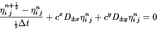
From (4.23) $\eta^{n+{ {\scriptscriptstyle \frac{1}{2}}}}_{i\;j}$ is obtained and further employed as boundary condition like in the water level BC (see Section 4.4.1).

On equation (4.23) $D_{\pm x}$ could represent D_-xwhen applied to the East border of the Domain or D_+x when used in the West boundary, and, similarly, $D_{\pm y}$ may be D_-y or D_+y.