Implicit implementation

Further evolution requested an implicit implementation of the low reflecting BC. It has been developed to be applied in the fully-implicit code introduced in Section 5.2.

To simplify we made the assumption that the surge leaving the computational domain always travels normal to the border.

For the row wise step we assume $\overrightarrow{c} =(c^x,0)$ and then:

$$\frac{\eta^{n+{\scriptscriptstyle \frac{1}{2}}}_{i\;j}-\eta^{... ...D_{\pm x}\eta^{n+{\scriptscriptstyle \frac{1}{2}}}_{i\;j} = 0$$ (7.21)

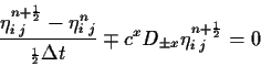
For the column wise step we assume $\overrightarrow{c} =(0,c^y)$ and then:

$$\frac{\eta^{n+1}_{i\;j}-\eta^{n+{\scriptscriptstyle \frac{1}{... ...ac{1}{2}}} \Delta t} \mp c^y D_{\pm y} \eta^{n+1}_{i\;j} = 0$$ (7.22)

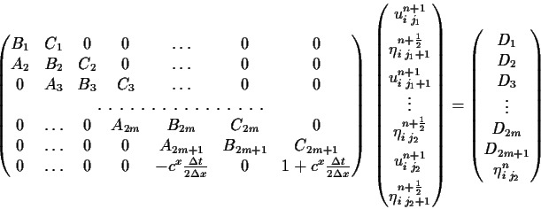
The above equations are included in the tri-diagonal system (4.26) giving the modified system. For instance, in the row wise iteration, assuming the West border has level-type boundary-condition and the East border corresponds to low-reflective condition, we get:

$$\begin{pmatrix} B_1&C_1&0&0&\dots&0&0\\ A_2&B_2&C_2&0&\dot... ...\vdots \\ D_{2m}\\ D_{2m+1} \\ \eta_{i\;j_2}^{n} \end{pmatrix}$$ (7.23)

A tridiagonal system is regained after performing an elimination step between the last two rows of (4.26). Then, the distributed tridiagonal solver is employed. We also obtain the boundary level $\eta_{i\;j_2+1}^{n+{\scriptstyle \frac{1}{2}}}$ from the solution, keeping the implicit nature of the model.