Line-wise i implicit sweep

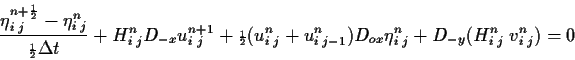
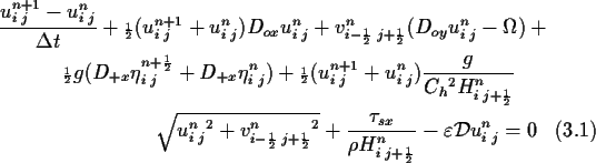
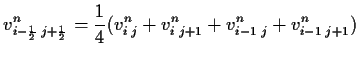
The equations (3.2)-(3.3) are approximated employing the finite differences operators defined in Section 4.2.3, as (over-line notation has been omitted):

$$\frac{\eta^{n+{\scriptscriptstyle \frac{1}{2}}}_{i\;j}-\eta^{... ... D_{ox} \eta^n_{i\;j}+ D_{-y} (H^n_{i\;j} \; v^n_{i\;j}) = 0$$ (7.2)

 $$\begin{multline}\frac{u^{n+1}_{i\;j} - u^{n}_{i\;j}} {\Delta t} + {\scriptscript... ...ptstyle \frac{1}{2}}}}} - \varepsilon \mathcal{D} u^n_{i\;j} = 0 \end{multline}$$

$$v^n_{i-{\scriptscriptstyle \frac{1}{2}}\;j+{\scriptscriptstyle \frac{1}{2}} } = \frac{1}{4} (v^n_{i\;j}+v^n_{i\;j+1}+v^n_{i-1\; j}+v^n_{i-1\; j+1})$$ (7.3)

$$H^n_{i\;j+{\scriptscriptstyle \frac{1}{2}}} = H_u + {\scriptscriptstyle \frac{1}{2}}(\eta^n_{i\;j} + \eta^n_{i\;j+1})$$ (7.4)

We use (4.2) at the center of the cell and (4.3) at the East side of the cell ( $\bigcirc{}$ and $\to{}$ respectively in figure 4.1) to solve $\eta^{n+{ {\scriptscriptstyle \frac{1}{2}}}}_{i\;j}$ and $u^{n+1}_{i\;j}$ for the i implicit sweep.